pacman::p_load(tmap, sf, sfdep, tidyverse, DT, leaflet)Take-home Exercise 1
0. Goals & Objectives.
On this page, we define Exploratory Spatial Data Analysis (ESDA) to understand spatial and spatio-temporal mobility patterns of public bus passengers in Singapore.
More detail about the task from: https://isss624-ay2023-24nov.netlify.app/take-home_ex01
Due to the nature of EDA and Data Analysis, parts of this page have been Collapsed or placed behind tabs, to avoid excessive scrolling.
For easier reading, this study is also presented in point-form.
0.1 Motivation
Public transport is a key concern for residents in land-scarce, population-dense Singapore. With COEs reaching record highs and authorities announcing the termination of bus services, there is no better time to understand the public transport network and systems in Singapore.
By understanding and modelling patterns of public transport consumption - including specifically Local Indicators of Spatial Association (LISA), insights can be provided to both public and private sector to formulate more informed decisions that for the benefit of the public, and not just for profit.
1. Geospatial Data Wrangling
This study was performed in R, written in R Studio, and published using Quarto.
1.1 Import Packages
This function calls pacman to load sf, tidyverse, tmap, knitr packages;
tmap: For thematic mapping; powerful mapping package;sf: for geospatial data handling, but also geoprocessing: buffer, point-in-polygon count, etc;sfdep: useful functions for creating weight matrix, LISA calculations etc;tidyverse: for non-spatial data handling; commonly used R package and containsdplyrfor dataframe manipulation andggplotfor data visualization;DT: for displaying datatables;leaflet: for custom layer controls overtmapvisualisations.
1.2 Import Data
1.2.1 Load Geospatial Bus Stop Data
- First, we load
BusStopshapefile data from LTA Datamall; st_read()is used to import the ESRI Shapefile data into ansfdataframe.
show code
raw_bus_stop_sf <- st_read(dsn = "data/geospatial",
layer = "BusStop") Reading layer `BusStop' from data source
`C:\1darren\ISSS624\Take-home_Ex01\data\geospatial' using driver `ESRI Shapefile'
Simple feature collection with 5161 features and 3 fields
Geometry type: POINT
Dimension: XY
Bounding box: xmin: 3970.122 ymin: 26482.1 xmax: 48284.56 ymax: 52983.82
Projected CRS: SVY21show code
head(raw_bus_stop_sf)Simple feature collection with 6 features and 3 fields
Geometry type: POINT
Dimension: XY
Bounding box: xmin: 13228.59 ymin: 30391.85 xmax: 41603.76 ymax: 44206.38
Projected CRS: SVY21
BUS_STOP_N BUS_ROOF_N LOC_DESC geometry
1 22069 B06 OPP CEVA LOGISTICS POINT (13576.31 32883.65)
2 32071 B23 AFT TRACK 13 POINT (13228.59 44206.38)
3 44331 B01 BLK 239 POINT (21045.1 40242.08)
4 96081 B05 GRACE INDEPENDENT CH POINT (41603.76 35413.11)
5 11561 B05 BLK 166 POINT (24568.74 30391.85)
6 66191 B03 AFT CORFE PL POINT (30951.58 38079.61)- We check the coordinate reference system with
st_crs();
st_crsReadout
show code
st_crs(raw_bus_stop_sf)Coordinate Reference System:
User input: SVY21
wkt:
PROJCRS["SVY21",
BASEGEOGCRS["WGS 84",
DATUM["World Geodetic System 1984",
ELLIPSOID["WGS 84",6378137,298.257223563,
LENGTHUNIT["metre",1]],
ID["EPSG",6326]],
PRIMEM["Greenwich",0,
ANGLEUNIT["Degree",0.0174532925199433]]],
CONVERSION["unnamed",
METHOD["Transverse Mercator",
ID["EPSG",9807]],
PARAMETER["Latitude of natural origin",1.36666666666667,
ANGLEUNIT["Degree",0.0174532925199433],
ID["EPSG",8801]],
PARAMETER["Longitude of natural origin",103.833333333333,
ANGLEUNIT["Degree",0.0174532925199433],
ID["EPSG",8802]],
PARAMETER["Scale factor at natural origin",1,
SCALEUNIT["unity",1],
ID["EPSG",8805]],
PARAMETER["False easting",28001.642,
LENGTHUNIT["metre",1],
ID["EPSG",8806]],
PARAMETER["False northing",38744.572,
LENGTHUNIT["metre",1],
ID["EPSG",8807]]],
CS[Cartesian,2],
AXIS["(E)",east,
ORDER[1],
LENGTHUNIT["metre",1,
ID["EPSG",9001]]],
AXIS["(N)",north,
ORDER[2],
LENGTHUNIT["metre",1,
ID["EPSG",9001]]]]- We see that although the projection is SVY21, the CRS (coordinate reference system) is EPSG 9001, which is incorrect;
- We thus use
st_set_crs()to set it to 3414, which is the EPSG code for SVY21;- we then use
st_crs()to confirm it is the correct EPSG code.
- we then use
st_crs Readout after st_transform
show code
raw_bus_stop_sf <- st_set_crs(raw_bus_stop_sf, 3414)Warning: st_crs<- : replacing crs does not reproject data; use st_transform for
thatshow code
st_crs(raw_bus_stop_sf)Coordinate Reference System:
User input: EPSG:3414
wkt:
PROJCRS["SVY21 / Singapore TM",
BASEGEOGCRS["SVY21",
DATUM["SVY21",
ELLIPSOID["WGS 84",6378137,298.257223563,
LENGTHUNIT["metre",1]]],
PRIMEM["Greenwich",0,
ANGLEUNIT["degree",0.0174532925199433]],
ID["EPSG",4757]],
CONVERSION["Singapore Transverse Mercator",
METHOD["Transverse Mercator",
ID["EPSG",9807]],
PARAMETER["Latitude of natural origin",1.36666666666667,
ANGLEUNIT["degree",0.0174532925199433],
ID["EPSG",8801]],
PARAMETER["Longitude of natural origin",103.833333333333,
ANGLEUNIT["degree",0.0174532925199433],
ID["EPSG",8802]],
PARAMETER["Scale factor at natural origin",1,
SCALEUNIT["unity",1],
ID["EPSG",8805]],
PARAMETER["False easting",28001.642,
LENGTHUNIT["metre",1],
ID["EPSG",8806]],
PARAMETER["False northing",38744.572,
LENGTHUNIT["metre",1],
ID["EPSG",8807]]],
CS[Cartesian,2],
AXIS["northing (N)",north,
ORDER[1],
LENGTHUNIT["metre",1]],
AXIS["easting (E)",east,
ORDER[2],
LENGTHUNIT["metre",1]],
USAGE[
SCOPE["Cadastre, engineering survey, topographic mapping."],
AREA["Singapore - onshore and offshore."],
BBOX[1.13,103.59,1.47,104.07]],
ID["EPSG",3414]]- We now do a quick plot to quickly visualize the bus stops;
qtm()is a wrapper to do a quick, simple plot usingtmapwithout defining arguments;- we use
tmap_mode("plot")to set the map as a static image, rather than as an interactive map, in order to save processing time.
show code
tmap_mode("plot")tmap mode set to plottingshow code
qtm(raw_bus_stop_sf)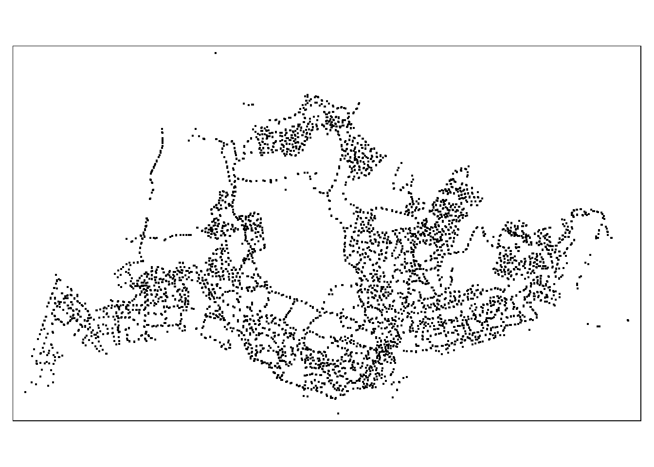
1.2.2 Visualizing Within Singapore’s Administrative National Boundary
- This image is hard to read; we can vaguely discern Singapore’s Southern coastline, but it can be hard to visualize.
- I have sourced and downloaded supplemental data about Singapore’s Administrative National Boundary (“SANB”) from igismap.com as a base layer for visualization;
- We set
tmap_mode("view")to allow us to scroll and confirm the SARB boundaries; - As before, we use
st_read()to load the shapefile data, andst_transform()to ensure the projection is correct;- We use
tm_shape() + tm_polygons()to map a grey layer of the SARB boundaries; - On top of which, we layer
tm_shape() + tm_dots()to show the bus stops.
- We use
- We set
show code
sanb_sf <- st_read(dsn = "data/geospatial",
layer = "singapore_administrative_national_boundary") %>%
st_transform(crs = 3414)Reading layer `singapore_administrative_national_boundary' from data source
`C:\1darren\ISSS624\Take-home_Ex01\data\geospatial' using driver `ESRI Shapefile'
Simple feature collection with 1 feature and 15 fields
Geometry type: MULTIPOLYGON
Dimension: XY
Bounding box: xmin: 103.6056 ymin: 1.158682 xmax: 104.4074 ymax: 1.471564
Geodetic CRS: WGS 84show code
tmap_mode("view")tmap mode set to interactive viewingshow code
tm_shape(sanb_sf) +
tm_polygons() +
tm_shape(raw_bus_stop_sf) +
tm_dots()show code
## Additional data from: Data.gov.sg, https://beta.data.gov.sg/datasets/d_02cba6aeeed323b5f6c723527757c0bc/viewThat’s because the Singapore National Administrative Boundaries map includes Pedra Branca, the much-disputed outlying island and easternmost point of Singapore.
It’s an amusing artifact here, but will not be involved in further analysis later.
- We note there are a number of bus stops outside Singapore’s boundaries; Specifically, three bus stops in a cluster just outside the Causeway, and one further North.
- We perform several steps to isolate & check the data;
- we use
st_filter()to find bus stops within Singapore’s Administrative National Boundaries, and createsg_bus_stop_sffor future use. - to check what bus stops have been dropped, we use
anti_join()to compareraw_bus_stop_sfwithsg_bus_stop_sf. We usest_drop_geometryon bothsfdataframes to only compare the non-geometry columns.
- we use
show code
sg_bus_stop_sf <- st_filter(raw_bus_stop_sf, sanb_sf)
anti_join(st_drop_geometry(raw_bus_stop_sf), st_drop_geometry(sg_bus_stop_sf))Joining with `by = join_by(BUS_STOP_N, BUS_ROOF_N, LOC_DESC)` BUS_STOP_N BUS_ROOF_N LOC_DESC
1 47701 NIL JB SENTRAL
2 46239 NA LARKIN TER
3 46609 NA KOTARAYA II TER
4 46211 NIL JOHOR BAHRU CHECKPT
5 46219 NIL JOHOR BAHRU CHECKPT- We see there are in fact 5 bus stops outside of Singapore (including the defunct Kotaraya II Terminal) that have been removed, which means our data cleaning was correct.
1.3 Geospatial Data Cleaning
1.3.1 Removing Duplicate Bus Stops
- But, do we need to do more data cleaning?
- We use
length()to find the total number of raw values in the$BUS_STOP_Ncolumn ofsg_bus_stop_sf;- We then compare this to
length(unique())to find the unique values;
- We then compare this to
- And, indeed, we find there are 16 bus stops that are repeated;
cat("Total number of rows in sg_bus_stop_sf\t\t: ", paste0(length(sg_bus_stop_sf$BUS_STOP_N)))Total number of rows in sg_bus_stop_sf : 5156cat("\nTotal unique bus stop IDs in sg_bus_stop_sf\t: ", paste0(length(unique(sg_bus_stop_sf$BUS_STOP_N))))
Total unique bus stop IDs in sg_bus_stop_sf : 5140cat("\nRepeated bus stops\t\t\t\t: ", paste0(length(raw_bus_stop_sf$BUS_STOP_N) - length(unique(raw_bus_stop_sf$BUS_STOP_N))))
Repeated bus stops : 16- It appears there are 16 datapoints that are specifically repeated; let’s identify the bus stop numbers with repeated rows:
- First we use
filter()with a pipe mark (usingorcondition) to identify repeated bus stop numbers (i.e.$BUS_STOP_N); - We sort them in ascending order using
arrange(); then, usinggroup_by()androw_number()we add row numbers based on$BUS_STOP_Nto a new column usingmutate().
- First we use
show code
repeated_df <- sg_bus_stop_sf %>%
filter(duplicated(BUS_STOP_N) | duplicated(BUS_STOP_N, fromLast = TRUE)) %>%
arrange(BUS_STOP_N) %>%
group_by(BUS_STOP_N) %>%
mutate(RowNumber = row_number())
datatable(repeated_df)- From examination, there are 32 bus stops sharing 16 bus stop numbers – 16 pairs of bus stops sharing the same number.
- Let’s examine these bus stop pairs on the map;
- we use
mapview()to display these repeated bus stops on the map; - we use
col="BUS_STOP_N"withpalette="Spectralto give each pair of bus stops an individual colour.
- we use
show code
tmap_mode("view")tmap mode set to interactive viewingshow code
tm_shape(sanb_sf) +
tm_polygons() +
tm_shape(repeated_df) +
tm_dots(col = "BUS_STOP_N", palette = "Spectral")- After confirming with Prof Kam, we will simply drop the second instance of the rows.
- we use
duplicated()to identify rows with repeated values of$BUS_STOP_N; duplicated rows will returnTRUEwhile all other rows will returnFALSE - We use
!to invert the values, so only the unduplicated rows will returnTRUE. - We then use square brackets
[]to indexsg_bus_stop_sfbased on the rows, and return only the unduplicated rows;
- we use
show code
sg_bus_stop_sf <- sg_bus_stop_sf[!duplicated(sg_bus_stop_sf$BUS_STOP_N), ]
head(sg_bus_stop_sf)Simple feature collection with 6 features and 3 fields
Geometry type: POINT
Dimension: XY
Bounding box: xmin: 13228.59 ymin: 30391.85 xmax: 41603.76 ymax: 44206.38
Projected CRS: SVY21 / Singapore TM
BUS_STOP_N BUS_ROOF_N LOC_DESC geometry
1 22069 B06 OPP CEVA LOGISTICS POINT (13576.31 32883.65)
2 32071 B23 AFT TRACK 13 POINT (13228.59 44206.38)
3 44331 B01 BLK 239 POINT (21045.1 40242.08)
4 96081 B05 GRACE INDEPENDENT CH POINT (41603.76 35413.11)
5 11561 B05 BLK 166 POINT (24568.74 30391.85)
6 66191 B03 AFT CORFE PL POINT (30951.58 38079.61)I was unable to take Prof Kam’s Data Analytics Lab, but I know of his fervour and attention to detail. I believe in informed choices, and so I performed manual cleaning with the following steps:
Remove the rows with lowercase names, as most
$LOC_DESCare in strict uppercaseRemove the rows with
NA$LOC_DESCRemove the row with
NIL$LOC_DESCFor remaining rows, drop second entry
Retain remaining rows
After this, we just run the same steps on sg_bus_stop_sf or perform an anti-join.
However, after clarification with Prof Kam, we just drop the second entry. My code is shown below for the gratification of those who may enjoy it.
show code
drop_second_stop = c("43709", "51071", "53041", "52059", "58031", "68091", "68099", "97079")
rows_to_retain_df <- repeated_df %>%
filter(
case_when(
BUS_STOP_N == "11009" & grepl("[a-z]", LOC_DESC) ~ FALSE,
BUS_STOP_N == "22501" & grepl("[a-z]", LOC_DESC) ~ FALSE,
BUS_STOP_N == "77329" & grepl("[a-z]", LOC_DESC) ~ FALSE,
BUS_STOP_N == "82221" & grepl("[a-z]", LOC_DESC) ~ FALSE,
BUS_STOP_N == "62251" & grepl("[a-z]", LOC_DESC) ~ FALSE,
BUS_STOP_N == "96319" & grepl("[a-z]", LOC_DESC) ~ FALSE,
BUS_STOP_N == "47201" & is.na(LOC_DESC) ~ FALSE,
BUS_STOP_N == "67421" & BUS_ROOF_N == "NIL" ~ FALSE,
BUS_STOP_N %in% drop_second_stop & RowNumber == 2 ~ FALSE,
TRUE ~ TRUE
)
)
rows_to_retain_df$LOC_DESC = toupper(rows_to_retain_df$LOC_DESC)
print("Printing rows to retain:")[1] "Printing rows to retain:"show code
rows_to_retain_dfSimple feature collection with 16 features and 4 fields
Geometry type: POINT
Dimension: XY
Bounding box: xmin: 13488.02 ymin: 32604.36 xmax: 44144.57 ymax: 47934
Projected CRS: SVY21 / Singapore TM
# A tibble: 16 × 5
# Groups: BUS_STOP_N [16]
BUS_STOP_N BUS_ROOF_N LOC_DESC geometry RowNumber
* <chr> <chr> <chr> <POINT [m]> <int>
1 11009 B04-TMNL GHIM MOH TER (23100.58 32604.36) 2
2 22501 B02 BLK 662A (13488.02 35537.88) 2
3 43709 B06 BLK 644 (18963.42 36762.8) 1
4 47201 NIL W'LANDS NTH STN (22632.92 47934) 2
5 51071 B21 MACRITCHIE RESERVO… (28311.27 36036.92) 1
6 52059 B03 OPP BLK 65 (30770.3 34460.06) 1
7 53041 B05 UPP THOMSON ROAD (28105.8 37246.76) 1
8 58031 UNK OPP CANBERRA DR (27089.69 47570.9) 1
9 62251 B03 BEF BLK 471B (35500.36 39943.34) 2
10 67421 B01 CHENG LIM STN EXIT… (34548.54 42052.15) 1
11 68091 B01 AFT BAKER ST (32164.11 42695.98) 1
12 68099 B02 BEF BAKER ST (32154.9 42742.82) 1
13 77329 B01 BEF PASIR RIS ST 53 (40765.35 39452.18) 1
14 82221 B01 BLK 3A (35323.6 33257.05) 1
15 96319 NIL YUSEN LOGISTICS (42187.23 34995.78) 2
16 97079 B14 OPP ST. JOHN'S CRES (44144.57 38980.25) 1- If we run the steps from above, we can see that there are no repeated bus stops.
cat("Total number of rows in sg_bus_stop_sf\t\t: ", paste0(length(sg_bus_stop_sf$BUS_STOP_N)))Total number of rows in sg_bus_stop_sf : 5140cat("\nTotal unique bus stop IDs in sg_bus_stop_sf\t: ", paste0(length(unique(sg_bus_stop_sf$BUS_STOP_N))))
Total unique bus stop IDs in sg_bus_stop_sf : 5140cat("\nRepeated bus stops\t\t\t\t: ", paste0(length(sg_bus_stop_sf$BUS_STOP_N) - length(unique(sg_bus_stop_sf$BUS_STOP_N))))
Repeated bus stops : 01.4 Generating Hexagon Maps
- We use
st_make_grid()withsquare = FALSEto create thehexagonlayer as defined in the study, which we nameraw_hex_grid;- We pass
cellsize = 500to create the hexagons of necessary size. Prof Kam defined the apothem as 250m, which means the distance between opposite edges is double that, or 500m;- I used
units::as_unitsto pass 500 metres into the argument. I am still uncertain whether a length of 500m needs to be reprojected, or whether we need to do any further transformation.
- I used
- We pass
- We use
st_sf()to convertraw_hex_gridinto ansfdataframe;mutate()is used here to create agrid_idcolumn;- We just use
st_transform()in case we need to reproject the coordinate system, just in case.
- However, trying to visualize this right now just gives us a map full of hexagons:
show code
raw_hex_grid = st_make_grid(sg_bus_stop_sf, cellsize = units::as_units(500, "m"), what = "polygons", square = FALSE) %>%
st_transform(crs = 3414)
# To sf and add grid ID
raw_hex_grid <- st_sf(raw_hex_grid) %>%
# add grid ID
mutate(grid_id = 1:length(lengths(raw_hex_grid))) %>%
st_transform(crs = 3414)
tmap_mode("plot")tmap mode set to plottingshow code
qtm(raw_hex_grid)
- What we will need is to isolate only the hexagons with bus stops in them.
- We use
lengths(st_intersects())to count the number of bus stops in each hexagon, and add that to a new column,$n_bus_stops; - We then create
hexagon_sfby filtering for only hexagons with non-zero bus stops in each.
- We use
- We then plot these using the usual
tmap()functions;tm_basemap()is used to create a “basemap” layer underneath to orient our hexagons.- We used OneMapSG as our comprehensive map of Singapore; if you zoom in, you can actually count the number of bus stops in red on the map.
show code
# Count number of points in each grid, code snippet referenced from:
# https://gis.stackexchange.com/questions/323698/counting-points-in-polygons-with-sf-package-of-r
raw_hex_grid$n_bus_stops = lengths(st_intersects(raw_hex_grid, sg_bus_stop_sf))
# remove grid without value of 0 (i.e. no points inside that grid)
hexagon_sf = filter(raw_hex_grid, n_bus_stops > 0)
# head(hexagon_sf)
tmap_mode("view")tmap mode set to interactive viewingshow code
tm_basemap(providers$OneMapSG.Grey) +
tm_shape(hexagon_sf) +
tm_fill(
col = "n_bus_stops",
palette = "-plasma",
style = "cont",
breaks = c(0, 1, 2, 3, 4, 5, 6, 7, 8, 9, 10, 11, 12),
title = "Number of bus_stops",
id = "grid_id",
showNA = FALSE,
alpha = 0.6,
popup.vars = c(
"Number of Bus Stops: " = "n_bus_stops"
),
popup.format = list(
n_bus_stops = list(format = "f", digits = 0)
)
) +
tm_borders(col = "grey40", lwd = 0.7)- There seem to be 2 regions of deep purple, centred over an area near, but not exactly over Pasir Ris and Choa Chu Kang MRTs.
- We perform some simple stats to count the total number of filtered hexagons, and to see the maximum number of bus stops in a hexagon.
show code
cat(paste("Total number of raw hexagons is\t\t\t: ", nrow(raw_hex_grid), "\n"))Total number of raw hexagons is : 5040 show code
cat(paste("Total number of hexagons (n_bus_stop > 1) is\t: ", nrow(hexagon_sf)), "\n")Total number of hexagons (n_bus_stop > 1) is : 1520 show code
cat("\nPrinting map_hexagon_sf:\n >> ")
Printing map_hexagon_sf:
>> show code
hexagon_sf[hexagon_sf$n_bus_stops > 10, ]Simple feature collection with 2 features and 2 fields
Geometry type: POLYGON
Dimension: XY
Bounding box: xmin: 17470.12 ymin: 38317.78 xmax: 42720.12 ymax: 40194.17
Projected CRS: SVY21 / Singapore TM
raw_hex_grid grid_id n_bus_stops
304 POLYGON ((17720.12 39616.82... 1584 11
1462 POLYGON ((42470.12 38317.78... 4355 11- For the next step, we’ll need to manage the aspatial bus trips dataset, which is what we’ll work on now.
1.5 Aspatial Data Wrangling: Bus trip dataset
1.5.1 Import Bus O/D Dataset
For our purposes, we will focus only on 2023-October Passenger Volume by Origin Destination Bus Stops, downloaded from LTA DataMall;
We use
read_csv()to load the data from the .csv file;We use
select()with a-sign to remove two columns redundant for our analysis:$PT_TYPEcolumn indicates the type of public transport, however, every value is “BUS”$YEAR_MONTHcolumn similarly has “2023-10” for every value, which we are aware of- With this in mind, we drop these two columns to save space.
Finally, we do
as.factor()to convert two columns ($ORIGIN_PT_CODEand$DESTINATION_PT_CODE)from character to factor, for easier analysis.
show code
odbus_2310 <- read_csv("data/aspatial/origin_destination_bus_202310.csv")Rows: 5694297 Columns: 7
── Column specification ────────────────────────────────────────────────────────
Delimiter: ","
chr (5): YEAR_MONTH, DAY_TYPE, PT_TYPE, ORIGIN_PT_CODE, DESTINATION_PT_CODE
dbl (2): TIME_PER_HOUR, TOTAL_TRIPS
ℹ Use `spec()` to retrieve the full column specification for this data.
ℹ Specify the column types or set `show_col_types = FALSE` to quiet this message.show code
odbus_2310 <- select(odbus_2310, -PT_TYPE, -YEAR_MONTH)
odbus_2310$ORIGIN_PT_CODE <- as.factor(odbus_2310$ORIGIN_PT_CODE)
odbus_2310$DESTINATION_PT_CODE <- as.factor(odbus_2310$DESTINATION_PT_CODE)
str(odbus_2310)tibble [5,694,297 × 5] (S3: tbl_df/tbl/data.frame)
$ DAY_TYPE : chr [1:5694297] "WEEKENDS/HOLIDAY" "WEEKDAY" "WEEKENDS/HOLIDAY" "WEEKDAY" ...
$ TIME_PER_HOUR : num [1:5694297] 16 16 14 14 17 17 17 7 14 14 ...
$ ORIGIN_PT_CODE : Factor w/ 5073 levels "01012","01013",..: 105 105 4428 4428 2011 834 834 781 4462 4462 ...
$ DESTINATION_PT_CODE: Factor w/ 5077 levels "01012","01013",..: 240 240 4742 4742 693 809 809 235 4002 4002 ...
$ TOTAL_TRIPS : num [1:5694297] 3 5 3 5 4 1 24 2 1 7 ...- This is a huge
tibbledataframe with over 5 million rows.
1.5.2 Filter For Peaks
- We now perform a multi-step filter process;
- We combine
mutate()withcase_when()to create a new column,$PEAK, based on the study criteria:- “WEEKDAY_MORNING_PEAK” if
$DAY_TYPEis “WEEKDAY” and bus tap-on time (e.g.$TIME_PER_HOUR) is between 6 am and 9 am, inclusive; - “WEEKDAY_AFTERNOON_PEAK” if
$DAY_TYPEis “WEEKDAY” and bus tap-on time (e.g.$TIME_PER_HOUR) is between 5 pm and 8pm, inclusive; - “WEEKEND_MORNING_PEAK” if
$DAY_TYPEis “WEEKENDS/HOLIDAY” and bus tap-on time (e.g.$TIME_PER_HOUR) is between 11 am and 2pm, inclusive; - “WEEKDAY_AFTERNOON_PEAK” if
$DAY_TYPEis “WEEKENDS/HOLIDAY” and bus tap-on time (e.g.$TIME_PER_HOUR) is between 4 pm and 7pm, inclusive; - Remaining values are assigned “Unknown” value.
- “WEEKDAY_MORNING_PEAK” if
- We then use
filter()to eliminate those with “Unknown”$PEAKvalues, i.e. rows outside the period of interest for the study - We use
group_by()to group the values by$ORIGIN_PT_CODEand$PEAK, and usesummarise()to aggregate the sum of$TOTAL_TRIPSas a new column,$TRIPS. - Finally, we use
pivot_wider()to pivot our long table into wide format, where each column represents one of the peak periods of interest in our study, and the values are filled from$TRIPS. We use thevalues_fillargument to fill in a value of “0” if the bus stop has a missing value. - We use
write_rds()to save the output dataframe,odbus_filtered, as an RDS object for future reference/load.
- We combine
- Note that we convert the values for
$TIME_PER_HOURto 24-hour clock, e.g. “5pm” is “17” hundred hours, “8pm” is “20” hundred hours,. - We truncate “Weekend/Public Holiday” to “WEEKEND” for easier reading/reference.
odbus_filtered <- odbus_2310 %>%
mutate(PEAK = case_when(
DAY_TYPE == "WEEKDAY" & TIME_PER_HOUR >= 6 & TIME_PER_HOUR <= 9 ~ "WEEKDAY_MORNING_PEAK",
DAY_TYPE == "WEEKDAY" & TIME_PER_HOUR >= 17 & TIME_PER_HOUR <= 20 ~ "WEEKDAY_AFTERNOON_PEAK",
DAY_TYPE == "WEEKENDS/HOLIDAY" & TIME_PER_HOUR >= 11 & TIME_PER_HOUR <= 14 ~ "WEEKEND_MORNING_PEAK",
DAY_TYPE == "WEEKENDS/HOLIDAY" & TIME_PER_HOUR >= 16 & TIME_PER_HOUR <= 19 ~ "WEEKEND_EVENING_PEAK",
TRUE ~ "Unknown"
)) %>%
filter(
case_when(
PEAK == "Unknown" ~ FALSE,
TRUE ~ TRUE
)) %>%
group_by(ORIGIN_PT_CODE, PEAK) %>%
summarise(TRIPS = sum(TOTAL_TRIPS)) %>%
pivot_wider(names_from = PEAK, values_from = TRIPS, values_fill = 0)`summarise()` has grouped output by 'ORIGIN_PT_CODE'. You can override using
the `.groups` argument.write_rds(odbus_filtered, "data/rds/odbus_filtered.rds")
head(odbus_filtered)# A tibble: 6 × 5
# Groups: ORIGIN_PT_CODE [6]
ORIGIN_PT_CODE WEEKDAY_AFTERNOON_PEAK WEEKDAY_MORNING_PEAK
<fct> <dbl> <dbl>
1 01012 8000 1770
2 01013 7038 841
3 01019 3398 1530
4 01029 9089 2483
5 01039 12095 2919
6 01059 2212 1734
# ℹ 2 more variables: WEEKEND_EVENING_PEAK <dbl>, WEEKEND_MORNING_PEAK <dbl>1.6 Combine Bus Trip Data With hexagon_sf Dataframe
- For our study purposes, we need to have the number of bus trips originating from each hexagon. In order to achieve this, we must combine our three current dataframes:
hexagon_sf, ansfdataframe with$grid_idcolumn (primary key) and the specific polygon geometry of each hexagon;sg_bus_stop_sf, ansfdataframe with the$BUS_STOP_N(primary key) and the point geometry of each bus stop;odbus_filtered, atibbledataframe with the$ORIGIN_PT_CODE(primary key) column and the trip details for each of the four peak periods of interest.
1.6.1 Identify Hexagon grid_id For Each Bus Stop
- First, we combine
hexagon_sfwithsg_bus_stop_sf;- We use
st_intersectionto combine the dataframes such that each row ofsg_bus_stop_sfhas an associatedgrid_id; - We use
select()to filter the resultantbus_stop_hexgrid_iddataframe to only$grid_idand$BUS_STOP_Ncolumns, and usest_drop_geometry()to convert into a simple dataframe with just two columns:
- We use
show code
bus_stop_hexgrid_id <- st_intersection(sg_bus_stop_sf, hexagon_sf) %>%
select(grid_id, BUS_STOP_N) %>%
st_drop_geometry()Warning: attribute variables are assumed to be spatially constant throughout
all geometriesshow code
cat("\nNumber of bus stops\t:", length(unique(bus_stop_hexgrid_id$BUS_STOP_N)))
Number of bus stops : 5140show code
cat("\nNumber of hexgrids\t:", length(unique(bus_stop_hexgrid_id$grid_id)))
Number of hexgrids : 1520show code
head(bus_stop_hexgrid_id) grid_id BUS_STOP_N
3265 31 25059
2566 59 25751
254 90 26379
2893 115 25761
2823 117 25719
4199 117 263891.6.2 Identify Bus Trip Details For Each Hexagon grid_id
- Here, we again use multiple steps to generate bus trip details for each hexagon
grid_id;- We use
left_join()to add thegrid_idto each row ofodbus_filtered, since each row has a unique single bus stop ID (i.e.$BUS_STOP_N); - We use
select()to retain only thegrid_idand the four peak-trips columns; - We combine
group_by()andsummarise()to aggregate the trips for each peak bygrid_id.
- We use
- Finally, we use
head()to preview thegrid_trips_dftibble dataframe.
show code
colnames(odbus_filtered)[1] "ORIGIN_PT_CODE" "WEEKDAY_AFTERNOON_PEAK" "WEEKDAY_MORNING_PEAK"
[4] "WEEKEND_EVENING_PEAK" "WEEKEND_MORNING_PEAK" show code
grid_trips_df <- left_join(odbus_filtered, bus_stop_hexgrid_id,
by = c("ORIGIN_PT_CODE" = "BUS_STOP_N")) %>%
select(grid_id,
WEEKDAY_MORNING_PEAK,
WEEKDAY_AFTERNOON_PEAK,
WEEKEND_MORNING_PEAK,
WEEKEND_EVENING_PEAK) %>%
group_by(grid_id) %>%
summarise(
WEEKDAY_MORNING_TRIPS = sum(WEEKDAY_MORNING_PEAK),
WEEKDAY_AFTERNOON_TRIPS = sum(WEEKDAY_AFTERNOON_PEAK),
WEEKEND_MORNING_TRIPS = sum(WEEKEND_MORNING_PEAK),
WEEKEND_EVENING_TRIPS = sum(WEEKEND_EVENING_PEAK)
)Adding missing grouping variables: `ORIGIN_PT_CODE`show code
head(grid_trips_df)# A tibble: 6 × 5
grid_id WEEKDAY_MORNING_TRIPS WEEKDAY_AFTERNOON_TRIPS WEEKEND_MORNING_TRIPS
<int> <dbl> <dbl> <dbl>
1 31 103 390 0
2 59 52 114 26
3 90 78 291 52
4 115 185 1905 187
5 117 1116 2899 455
6 118 53 241 76
# ℹ 1 more variable: WEEKEND_EVENING_TRIPS <dbl>1.6.3 Combine Bus Trip Details Back Into hexagon_sf
- Finally, it’s time to recombine bus trip data back into
hexagon_sf;- We use
left_joinon$grid_idto add trip data back into hexagon_sf; - We add a failsafe
mutate()to replace any “NA” values for the columns.
- We use
show code
hexagon_sf <- left_join(hexagon_sf, grid_trips_df,
by = 'grid_id' ) %>%
mutate(
WEEKDAY_MORNING_TRIPS = ifelse(is.na(WEEKDAY_MORNING_TRIPS), 0, WEEKDAY_MORNING_TRIPS),
WEEKDAY_AFTERNOON_TRIPS = ifelse(is.na(WEEKDAY_AFTERNOON_TRIPS), 0, WEEKDAY_AFTERNOON_TRIPS),
WEEKEND_MORNING_TRIPS = ifelse(is.na(WEEKEND_MORNING_TRIPS), 0, WEEKEND_MORNING_TRIPS),
WEEKEND_EVENING_TRIPS = ifelse(is.na(WEEKEND_EVENING_TRIPS), 0, WEEKEND_EVENING_TRIPS),
)
head(hexagon_sf)Simple feature collection with 6 features and 6 fields
Geometry type: POLYGON
Dimension: XY
Bounding box: xmin: 3720.122 ymin: 27925.48 xmax: 4970.122 ymax: 31533.92
Projected CRS: SVY21 / Singapore TM
grid_id n_bus_stops WEEKDAY_MORNING_TRIPS WEEKDAY_AFTERNOON_TRIPS
1 31 1 103 390
2 59 1 52 114
3 90 1 78 291
4 115 1 185 1905
5 117 2 1116 2899
6 118 1 53 241
WEEKEND_MORNING_TRIPS WEEKEND_EVENING_TRIPS raw_hex_grid
1 0 56 POLYGON ((3970.122 27925.48...
2 26 14 POLYGON ((4220.122 28358.49...
3 52 100 POLYGON ((4470.122 30523.55...
4 187 346 POLYGON ((4720.122 28358.49...
5 455 634 POLYGON ((4720.122 30090.54...
6 76 55 POLYGON ((4720.122 30956.57...1.7 Exploratory Data Analysis Of Bus Trips, Across Peak Periods, By Hexagons
- For
ggplot, we need data in long format, so we can usegather()ongrid_trips_dffrom Section 1.6.2 to pivot this; - We then pipe this into a
geom_boxplot()for an exploratory look:
show code
gather(grid_trips_df, key = "Peak", value = "Trips", -grid_id) %>%
ggplot( aes(x=Peak, y=Trips, fill=Peak)) +
geom_boxplot() +
ggtitle("Boxplot: Trips over peak periods, 2023-Oct data") +
xlab("") +
theme(
legend.position="none"
) +
coord_flip()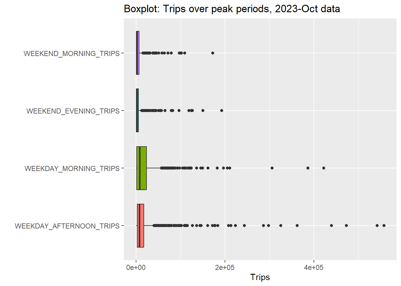
We also observe that number of trips for Weekday Morning & Weekday Afternoon seems to be larger than Weekend Morning and Weekend Evening peak trips. This is also confirmed by the figure in the next section.
This means that we will have to consider Weekday and Weekend peaks on different scales.
- This is an exceptionally ugly plot, but it shows an important point: there is some serious right skew in our dataset;
- Clearly, there are some hexagons with exceptionally high trips compared to the rest of the hexagons But, could this be because some hexagons have up to 11 bus stops, while others have 1 or 2?
- We do a quick scatter plot based on
$n_bus_stopsto verify this:
show code
hexagon_sf %>%
st_drop_geometry() %>%
pivot_longer(cols = starts_with("WEEK"),
names_to = "PEAK", values_to = "TRIPS") %>%
ggplot( aes(x=TRIPS, y=n_bus_stops, color=PEAK, shape=PEAK)) +
geom_point(size=2) +
ggtitle("Scatterplot: Trips over peak periods by number of bus stops per hexagon, 2023-Oct data") +
theme(legend.position=c(.85, .15),
legend.background = element_rect(fill = "transparent"),
legend.key.size = unit(0.5, "cm"),
legend.text = element_text(size = 6),
legend.title = element_text(size = 8)
) 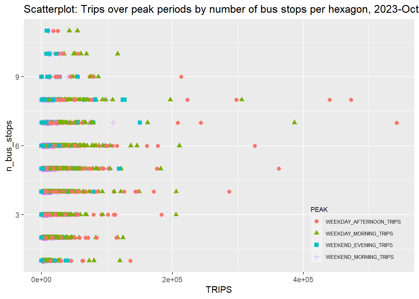
- Surprising results from our plot! If we consider those with > 100,000 trips as outliers, most of them come from hexagons with between 4-8 bus stops;
- There is some correlation between number of bus stops and high numbers of trips, but a stronger factor is peak time; Weekday Morning peak trips, followed by Weekday Afternoon peak trips, contribute to the largest outliers.
I note that these visualizations only scrape the surface of understanding the data. However, this is not the focus of our study; we do these quick visualizations only to provide better context for our study.
2 Geovisualisation And Geocommunication
2.1 Passenger Trips By Origin At Hexagon Level
- We use
datatable()to displayhexagon_sfas an interactive table. NB: In order to view the position ofgrid_id, we’ll need to look at the next section.
show code
datatable(hexagon_sf)2.2 Visualising The Geographical Distribution Of Passenger Trips By Origin At Hexagon Level
The below code block is a little more complicated, but can be thought of as combining a tm object with custom tm_leaflet() settings:
Creating the tm object:
- We start with
tmap_mode("view")to create an interactive base layer of Singapore; - To create the “WEEKDAY_MORNING_TRIPS” layer, we perform the following:
- We use
tm_shape()andtm_borders()to visualize the hexagons inhexagon_sf; - We use
tm_filland pass the argumentcol = "WEEKDAY_MORNING_TRIPS"to colour each hexagon based on the number of trips in the$WEEKDAY_MORNING_TRIPScolumn; - Since we are largely comparing the patterns, we use
style = "jenks"to make use of the Jenks natural breaks classification method to group the number of trips in different hexagons. This results in more visually distinct clusters that allow us to better spot patterns and distribution. - This also means that each layer will be on a different scale; we therefore use different
palettesso the user understand the scale breaks on each layer is different. For consistency, we also match each layer with the colourscheme in the visualisations in section 1.6.4. - For each feature, we add the
group="WEEKDAY_MORNING_TRIPS"argument for leaflet control later.
- We use
- We repeat this for the other three layers as well.
Creating the tm_leaflet controls:
- We use
addLayersControl()to specify the checkbox-menu ofoverlayGroups, according to the four defined peaks. Additional arguments allow us to ensure the menu is positioned at the top-left and expanded, for visibility and ease of use.
show code
tmap_mode("view")tmap mode set to interactive viewingshow code
tm <- tm_shape(hexagon_sf, group="WEEKDAY_MORNING_TRIPS") +
tm_borders(group="WEEKDAY_MORNING_TRIPS") +
tm_fill(col = "WEEKDAY_MORNING_TRIPS",
palette = "Greens",
style = "jenks",
group="WEEKDAY_MORNING_TRIPS") +
tm_shape(hexagon_sf, group="WEEKDAY_AFTERNOON_TRIPS") +
tm_borders(group="WEEKDAY_AFTERNOON_TRIPS") +
tm_fill(col = "WEEKDAY_AFTERNOON_TRIPS",
palette = "Reds",
style = "jenks",
group="WEEKDAY_AFTERNOON_TRIPS") +
tm_shape(hexagon_sf, group="WEEKEND_MORNING_TRIPS") +
tm_borders(group="WEEKEND_MORNING_TRIPS") +
tm_fill(col = "WEEKEND_MORNING_TRIPS",
palette = "Blues",
style = "jenks",
group="WEEKEND_MORNING_TRIPS") +
tm_shape(hexagon_sf, group="WEEKEND_EVENING_TRIPS") +
tm_borders(group="WEEKEND_EVENING_TRIPS") +
tm_fill(col = "WEEKEND_EVENING_TRIPS",
palette = "Purples",
style = "jenks",
group="WEEKEND_EVENING_TRIPS")
tm %>%
tmap_leaflet() %>%
hideGroup(c("WEEKDAY_AFTERNOON_TRIPS", "WEEKEND_MORNING_TRIPS", "WEEKEND_EVENING_TRIPS")) %>%
addLayersControl(
overlayGroups = c("WEEKDAY_MORNING_TRIPS", "WEEKDAY_AFTERNOON_TRIPS",
"WEEKEND_MORNING_TRIPS", "WEEKEND_EVENING_TRIPS"),
options = layersControlOptions(collapsed = FALSE),
position = "topleft"
)show code
## Code referenced from: https://stackoverflow.com/questions/53094379/in-r-tmap-how-do-i-control-layer-visibility-in-interactive-mode2.3 Observed Spatial Patterns
There are three major patterns observable from the geospatial visualization. First, we note that a minority of hexagons are responsible for a majority of trips. Most hexagons fall within the first quintile of trips made. However, across all peak periods, we can observe contiguous regions of deeply-coloured hexagons (by switching between layers in the above visualisation) that represent regions with high numbers of bus trips. This suggests the presence of transport hubs where commuters congregate to take bus trips during peak hours – possibly bus interchanges, or MRT stations.
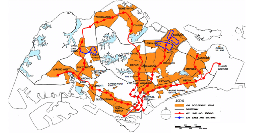
Secondly, we observe that these regions of high bus trips seem to roughly correspond to regions of residential new towns and MRT lines (see image below). This makes sense, as commuters are likely to leave their homes in the mornings or take buses from MRT stations. We also see a darker region in the WEEKDAY_AFTERNOON_TRIPS map corresponding to the Central Business District, as commuters leave their workplace back to home.
Finally, however, we observe that there is incomplete information. There are more trips on Weekday Afternoons compared to Weekday Mornings, and more trips on Weekdays than Weekends. This is likely due to other forms of transport (e.g. private cars, MRTs, bicycles).
- We can also visualize the map of all four on the same scale, for side-by-side comparison;
- However, as has been noted, the difference in scales between Weekday (left column) and Weekend (right column) trips means that there’s not much visual information value; the Weekend plot looks mostly flat.
- We will not go into detail about the code or spatial patterns, aside from noting that the hexagons with the highest number of trips are the same on weekdays and weekends, across morning and afternoon/evening peaks.
show code
tmap_mode("plot")tmap mode set to plottingshow code
custom_breaks <- seq(0, 550000, by = 50000)
wd_morn <- tm_shape(hexagon_sf) +
tm_fill("WEEKDAY_MORNING_TRIPS",
style = "cont",
palette = "-plasma",
breaks = custom_breaks,
title = "Trips") +
tm_borders() +
tm_layout(title = "WEEKDAY_MORNING", title.size = 0.8, legend.show = FALSE)
wd_aft <- tm_shape(hexagon_sf) +
tm_fill("WEEKDAY_AFTERNOON_TRIPS",
style = "cont",
palette = "-plasma",
breaks = custom_breaks,
title = "Trips") +
tm_borders() +
tm_layout(title = "WEEKDAY_AFTERNOON", title.size = 0.8, legend.show = FALSE)
we_morn <- tm_shape(hexagon_sf) +
tm_fill("WEEKEND_MORNING_TRIPS",
style = "cont",
palette = "-plasma",
breaks = custom_breaks,
title = "Trips") +
tm_borders() +
tm_layout(title = "WEEKEND_MORNING", title.size = 0.8, legend.show = FALSE)
we_eve <- tm_shape(hexagon_sf) +
tm_fill("WEEKEND_EVENING_TRIPS",
style = "cont",
palette = "-plasma",
breaks = custom_breaks,
title = "Trips") +
tm_borders() +
tm_layout(title = "WEEKEND_EVENING", title.size = 0.8, legend.text.size = 0.5)
tmap_arrange(wd_morn, we_morn, wd_aft, we_eve)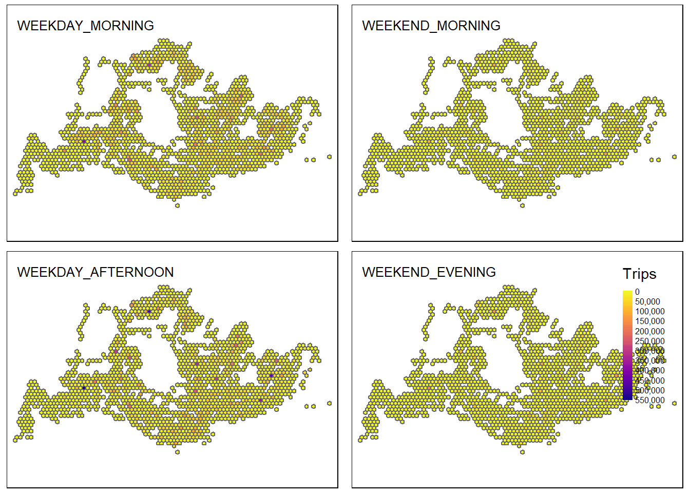
3. Geospatial Analysis: Local Indicators of Spatial Association (LISA) Analysis
3.1 Visualizing Queen Contiguity (And Why It Won’t Work)
- To perform LISA analysis, we will need an
nbmatrix. - However, using QUEEN contiguity will not work, as there are a number of hexagons without neighbours (i.e. no adjacent/touching hexagons);
- This is visible if we call
st_contiguity()on ourhexagon_sfwith the argument “queen=TRUE” for QUEEN contiguity;- We see “9 regions with no links”, i.e. 9 hexagons will have no neighbours.
show code
wm_hex <- st_contiguity(hexagon_sf, queen=TRUE)
summary(wm_hex)Neighbour list object:
Number of regions: 1520
Number of nonzero links: 6874
Percentage nonzero weights: 0.2975242
Average number of links: 4.522368
9 regions with no links:
561 726 980 1047 1415 1505 1508 1512 1520
Link number distribution:
0 1 2 3 4 5 6
9 39 109 205 291 364 503
39 least connected regions:
1 7 22 38 98 169 187 195 211 218 258 259 264 267 287 454 562 607 642 696 708 732 751 784 869 1021 1022 1046 1086 1214 1464 1471 1482 1500 1501 1503 1506 1510 1519 with 1 link
503 most connected regions:
10 13 16 17 24 25 31 35 42 43 48 53 55 60 63 67 73 77 80 81 84 85 87 88 91 92 97 102 107 111 117 121 127 133 140 141 143 148 149 150 154 155 156 157 163 164 165 173 174 175 183 184 185 191 192 193 194 200 201 202 205 206 207 208 216 229 239 243 244 246 257 266 271 278 279 283 284 291 292 298 300 301 302 304 309 310 312 313 316 321 324 325 327 337 338 339 340 343 352 355 363 368 390 391 400 402 403 407 414 418 423 425 431 436 437 438 440 443 450 451 452 461 466 467 468 469 473 477 480 481 485 489 493 494 496 502 503 507 513 514 517 518 523 529 534 539 543 548 549 550 552 556 558 564 568 573 574 576 577 581 590 591 594 598 599 604 605 609 615 619 624 626 633 636 637 638 648 649 650 654 655 657 658 659 669 670 671 677 680 681 682 687 688 690 691 700 701 704 705 706 713 716 717 724 727 728 729 740 741 755 757 758 760 771 774 775 776 777 782 783 787 788 789 792 793 794 795 799 800 806 807 810 811 812 813 819 820 823 824 825 830 831 832 841 843 844 846 847 848 850 851 852 853 854 860 863 865 866 867 871 872 876 877 878 880 881 882 884 885 887 888 891 893 896 899 902 905 906 910 914 919 921 926 927 928 930 931 935 937 943 944 945 946 947 948 954 958 959 962 963 968 969 971 972 973 977 984 985 986 987 988 990 996 997 998 999 1004 1011 1012 1013 1014 1024 1025 1026 1028 1029 1036 1037 1038 1042 1050 1051 1054 1056 1057 1062 1063 1064 1066 1067 1068 1069 1076 1078 1079 1080 1083 1089 1093 1100 1101 1102 1105 1106 1110 1111 1117 1120 1121 1122 1128 1133 1134 1135 1136 1141 1142 1144 1145 1146 1147 1148 1150 1156 1157 1158 1162 1163 1164 1166 1169 1170 1171 1172 1176 1177 1178 1179 1180 1184 1186 1190 1191 1192 1193 1194 1201 1202 1203 1204 1205 1206 1207 1210 1211 1217 1218 1219 1220 1221 1227 1233 1234 1235 1239 1244 1245 1251 1253 1254 1255 1261 1265 1266 1271 1272 1273 1277 1281 1283 1289 1299 1301 1302 1303 1304 1316 1318 1324 1325 1326 1327 1329 1330 1331 1334 1335 1336 1337 1343 1344 1345 1352 1353 1355 1356 1361 1365 1366 1368 1369 1371 1372 1377 1380 1381 1382 1384 1388 1391 1393 1395 1398 1406 1408 1412 1417 1418 1420 1424 1425 1426 1427 1428 1433 1434 1435 1436 1440 1441 1442 1446 1447 1449 1451 1453 1456 1457 1459 1460 1461 1462 1469 with 6 linksWe can perform a quick visualization of the hexagons with no neighbours;
We plot all hexagons, in green, from
hexagon_sf, as an underlying layer;On top of this layer, we plot all hexagons with no neighbours,
hexagon_sf_nonbin red;- Using the output from above, we create a list of hexagons with no neighbours,
hex_no_nb; - We create
hexagon_sf_nonbby adding a$RowNumbercolumn usingmutate()and usingrow_number()to label each row; - Finally, we use
subset()to select only the hexagons with no neighbours.
show code
hex_no_nb <- c(561, 726, 980, 1047, 1415, 1505, 1508, 1512, 1520) hexagon_sf_nonb <- hexagon_sf %>% mutate(RowNumber = row_number()) %>% subset((RowNumber %in% hex_no_nb)) tm_shape(hexagon_sf) + tm_fill("green") + tm_borders() + tm_shape(hexagon_sf_nonb) + tm_fill("red")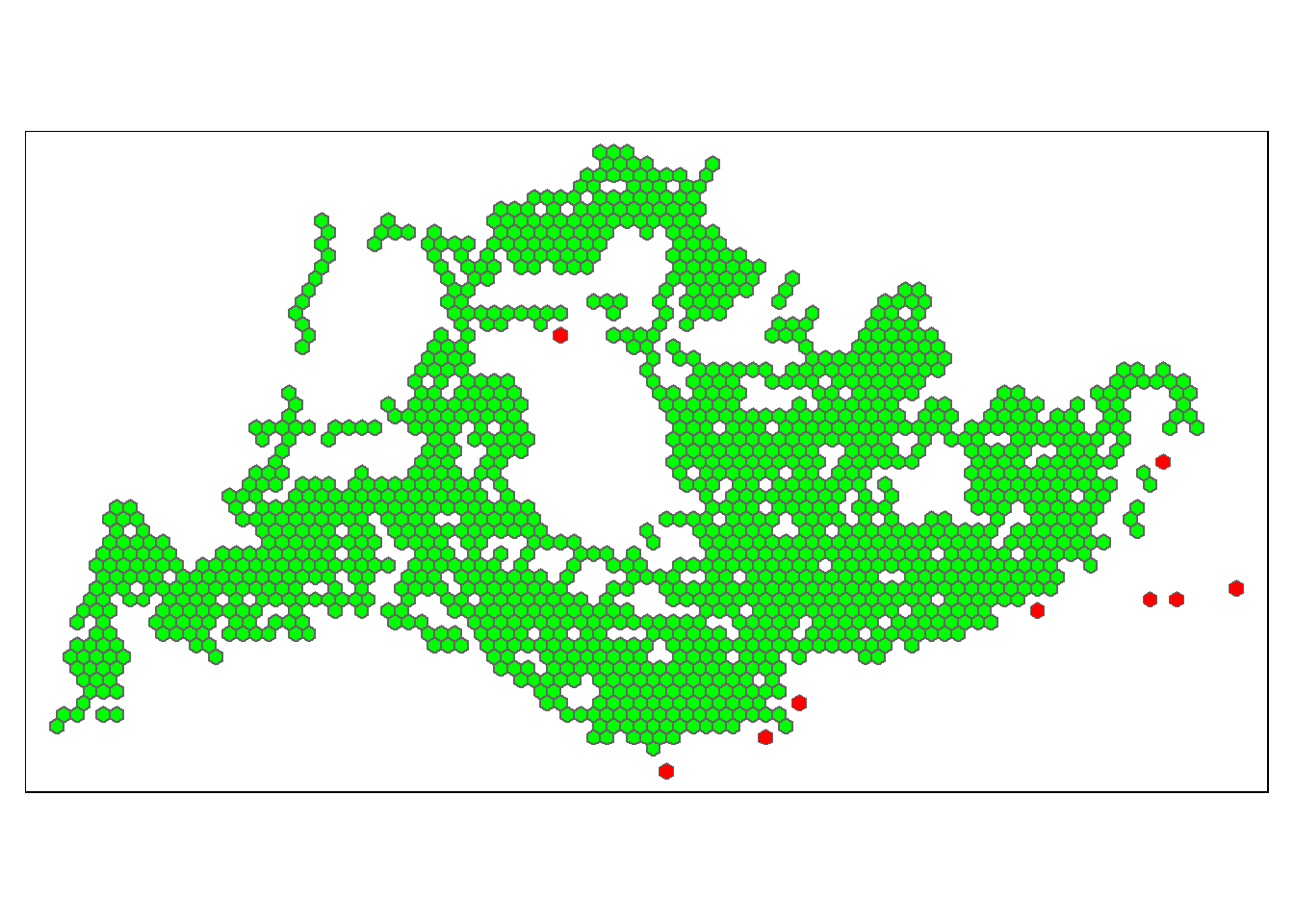
- Using the output from above, we create a list of hexagons with no neighbours,
We note that the Easternmost red outlier hexagon is likely the bus stop outside Changi Naval Base:
show code
coordinates <- st_coordinates(raw_bus_stop_sf$geometry)
# Find the index of the easternmost point
easternmost_index <- which.max(coordinates[, 1])
# Extract the easternmost bus-stop
easternmost_point <- raw_bus_stop_sf[easternmost_index, ]
easternmost_point # 96439Simple feature collection with 1 feature and 3 fields
Geometry type: POINT
Dimension: XY
Bounding box: xmin: 48284.56 ymin: 33326.57 xmax: 48284.56 ymax: 33326.57
Projected CRS: SVY21 / Singapore TM
BUS_STOP_N BUS_ROOF_N LOC_DESC geometry
3063 96439 B04 CHANGI NAVAL BASE POINT (48284.56 33326.57)3.2 Creating Distance-Based nb Neighbours Matrix
3.2.1 Identifying Coordinates Of centroid
- Creating Distance-based neighbour weights matrix relies on point geometry;
- That means, we need to calculate the centroids of each hexagon, by creating
centroid_coords:- This combines two lists,
longitudeandlatitude, which we extract usingst_centroidand indexing either the first or second value using[[]] map_dbl()ensures we obtainlongitudeandlatitudeas double integers
- This combines two lists,
show code
longitude <- map_dbl(hexagon_sf$raw_hex_grid, ~st_centroid(.x)[[1]])
latitude <- map_dbl(hexagon_sf$raw_hex_grid, ~st_centroid(.x)[[2]])
centroid_coords <- cbind(longitude, latitude)
cat("Printing first 6 rows of `centroid_coords`:\n")Printing first 6 rows of `centroid_coords`:show code
head(centroid_coords) longitude latitude
[1,] 3970.122 28214.15
[2,] 4220.122 28647.16
[3,] 4470.122 30812.23
[4,] 4720.122 28647.16
[5,] 4720.122 30379.22
[6,] 4720.122 31245.243.2.2 Identifying The Minimum DIstance So Each Hexagon Has At Least One Neighbour
- We use
st_knn()with argument “k=1” to create a neighbour list,k1_nn_obj, such that each hexagon centroid has 1 neighbour (using the k-nearest-neighbour algorithm); - We use
st_nb_dists()to create a list of distances between each hexagon centroid and its nearest neighbours; - We performing
unlist()on the object to convert it into a vector of numeric values, so that we can runsummary()to see summary statistics on it.
show code
k1_nn_obj <- st_knn(centroid_coords, k = 1)
k1dists <- unlist(st_nb_dists(centroid_coords, k1_nn_obj))
summary(k1dists) Min. 1st Qu. Median Mean 3rd Qu. Max.
500.0 500.0 500.0 503.4 500.0 2291.3 - We see that the furthest distance between a hexagon and its nearest neighbour is about 2.3km away; that will be the upper limit value needed to create distance-based contiguity.
Personally, I would drop the outlier (the hexagon with the Changi Naval Base bus stop). My reasoning is thus:
Logically speaking, we are enmeshing regions up to more than four hexagons away; this may lea to greater-than-average lag than is necessary.
As a commuter, walking 2.3km to the next nearest bus-stop hexagon is impractical and a clear outlier situation.
In personal testing, removing Changi Naval Base drops the maximum nearest-neighbour distance to 1km, which is more reasonable for both analysis and real-life considerations, but I note this here for future work and as commentary.
3.3 Creating A Distance-Based Weights Natrix
- To create a neighbours list, we use
st_dist_band()on thecentroid_coordsof our hexagons, and pass “upper = 2300” to set the upper limit for the neighbour threshold (rounding up to 2.3km from our previous result); - We then use
st_weights()to create the weights matrix; by default, the function creates row-standardised weights, but we could also have specified “style =”W”” for completeness.
show code
hex_2km_nb <- st_dist_band(centroid_coords, lower = 0, upper = 2300)
hex_2km_wt <- st_weights(hex_2km_nb)
head(hex_2km_wt, 5)[[1]]
[1] 0.1 0.1 0.1 0.1 0.1 0.1 0.1 0.1 0.1 0.1
[[2]]
[1] 0.0625 0.0625 0.0625 0.0625 0.0625 0.0625 0.0625 0.0625 0.0625 0.0625
[11] 0.0625 0.0625 0.0625 0.0625 0.0625 0.0625
[[3]]
[1] 0.03448276 0.03448276 0.03448276 0.03448276 0.03448276 0.03448276
[7] 0.03448276 0.03448276 0.03448276 0.03448276 0.03448276 0.03448276
[13] 0.03448276 0.03448276 0.03448276 0.03448276 0.03448276 0.03448276
[19] 0.03448276 0.03448276 0.03448276 0.03448276 0.03448276 0.03448276
[25] 0.03448276 0.03448276 0.03448276 0.03448276 0.03448276
[[4]]
[1] 0.05555556 0.05555556 0.05555556 0.05555556 0.05555556 0.05555556
[7] 0.05555556 0.05555556 0.05555556 0.05555556 0.05555556 0.05555556
[13] 0.05555556 0.05555556 0.05555556 0.05555556 0.05555556 0.05555556
[[5]]
[1] 0.03333333 0.03333333 0.03333333 0.03333333 0.03333333 0.03333333
[7] 0.03333333 0.03333333 0.03333333 0.03333333 0.03333333 0.03333333
[13] 0.03333333 0.03333333 0.03333333 0.03333333 0.03333333 0.03333333
[19] 0.03333333 0.03333333 0.03333333 0.03333333 0.03333333 0.03333333
[25] 0.03333333 0.03333333 0.03333333 0.03333333 0.03333333 0.033333333.4 Calculate Local Moran’s I
- For each peak period, we perform a calculation using
local_moran(), feeding in thenbneighbours list andwtweight matrix from the previous section;- We use
select()to isolate the columns that we need, specifically the Local Moran’s I statistics$ii, the p-value$p_ii, and the LISA$mean(here, we use mean over median or pysal columns); - For ease of use later, we rename these columns with
rename(); - We repeat for each of the four peak periods.
- We use
- Finally, we use a
cbind()to append the columns back to ourhexagon_sf:
show code
localMI_day_morn <- local_moran(hexagon_sf$WEEKDAY_MORNING_TRIPS, hex_2km_nb, hex_2km_wt) %>%
select(ii, p_ii, mean) %>%
rename(DAY_MORN_LMI = ii,
DAY_MORN_p = p_ii,
DAY_MORN_mean = mean)
localMI_day_aft <- local_moran(hexagon_sf$WEEKDAY_AFTERNOON_TRIPS, hex_2km_nb, hex_2km_wt) %>%
select(ii, p_ii, mean) %>%
rename(DAY_AFT_LMI = ii,
DAY_AFT_p = p_ii,
DAY_AFT_mean = mean)
localMI_end_morn <- local_moran(hexagon_sf$WEEKEND_MORNING_TRIPS , hex_2km_nb, hex_2km_wt) %>%
select(ii, p_ii, mean) %>%
rename(END_MORN_LMI = ii,
END_MORN_p = p_ii,
END_MORN_mean = mean)
localMI_end_eve <- local_moran(hexagon_sf$WEEKEND_EVENING_TRIPS, hex_2km_nb, hex_2km_wt) %>%
select(ii, p_ii, mean) %>%
rename(END_EVE_LMI = ii,
END_EVE_p = p_ii,
END_EVE_mean = mean)
hexagon_sf_local_moran <- cbind(hexagon_sf,localMI_day_morn, localMI_day_aft, localMI_end_morn, localMI_end_eve)show code
datatable(hexagon_sf_local_moran)3.5 Removing Statistically Non-Significant Values Before Plotting the LISA Map
- To plot the LISA map, we will use the peak-specific
$meancolumn; this uses the mean of values to classify regions into either outliers (High-Low or Low-High) or clusters (High-High or Low-Low). - However, we also only want to see categories if they are statistically significant, i.e. if the
$p_iivalue is >= 0.05, we should coerce the LISA category to “Insignificant”, so we need to do some cleaning; - Once again, we use our trusty friend
mutate()to modify existing columns;- We pass the column
$DAY_MORN_meanand define acase_when()statement that replaces the value with “Insignificant” if the$DAY_MORN_pvalue is greater than 0.05 (i.e. p-value is higher than 0.05); - We repeat this for the other peak periods:
- We pass the column
show code
df <- hexagon_sf_local_moran %>%
mutate(
DAY_MORN_mean = case_when(
DAY_MORN_p >= 0.05 ~ "Insignificant",
TRUE ~ DAY_MORN_mean
),
DAY_AFT_mean = case_when(
DAY_AFT_p >= 0.05 ~ "Insignificant",
TRUE ~ DAY_AFT_mean
),
END_MORN_mean = case_when(
END_MORN_p >= 0.05 ~ "Insignificant",
TRUE ~ END_MORN_mean
),
END_EVE_mean = case_when(
END_EVE_p >= 0.05 ~ "Insignificant",
TRUE ~ END_EVE_mean
)
)
datatable(head(df))3.6 Plotting The LISA Map
- Now, we perform a similar plot to the visualisation above in Section 2.2;
- We use
tmap_leaflet()andaddLayersControl()to allow for toggling between the various peak periods; - We pass
group=argument for eachtmapfunction to group them into layer groups; - We use
tm_shape()to plot the hexagons,tm_borders()to draw the borders andtm_fill()to colour them in.
- We use
- The difference here is we define a custom palette,
colors, sourced from Prof Kam’s book.
show code
tmap_mode("view")tmap mode set to interactive viewingshow code
colors <- c("#2c7bb6", "#abd9e9", "#ffffff", "#fdae61", "#d7191c")
# Custom colors palette sourced from: https://r4gdsa.netlify.app/chap10#plotting-lisa-map
tm2 <- tm_shape(df, group="DAY_MORN") +
tm_borders(group="DAY_MORN") +
tm_fill(col = "DAY_MORN_mean",
alpha = 0.8,
palette = colors,
group="DAY_MORN") +
tm_shape(df, group="DAY_AFT") +
tm_borders(group="DAY_AFT") +
tm_fill(col = "DAY_AFT_mean",
alpha = 0.8,
palette = colors,
group="DAY_AFT") +
tm_shape(df, group="END_MORN") +
tm_borders(group="END_MORN") +
tm_fill(col = "END_MORN_mean",
alpha = 0.8,
palette = colors,
group="END_MORN") +
tm_shape(df, group="END_EVE") +
tm_borders(group="END_EVE") +
tm_fill(col = "END_EVE_mean",
alpha = 0.8,
palette = colors,
group="END_EVE")
tm2 %>%
tmap_leaflet() %>%
hideGroup(c("DAY_AFT", "END_MORN", "END_EVE")) %>%
addLayersControl(
overlayGroups = c("DAY_MORN", "DAY_AFT",
"END_MORN", "END_EVE"),
options = layersControlOptions(collapsed = FALSE),
position = "topleft"
) - The Westmost region (Tuas, Boon Lay) areas are hugely underserved by buses, across all peak periods.
- Travel patterns on Weekends are more homogeneous (regions are similar across Weekend Morning and Weekend Evening peaks); however, there is a stark difference between Weekday Morning and Weekday Afternoon peaks. This likely reflects people leaving homes to commute / people leaving places of work, study, or commerce to return home.
- Across all peak periods, there are consistent areas of high demand; these include:
- A region in the West, stretching across Jurong West-Jurong East-Bukit Batok-Choa Chu Kang neighbourhoods;
- A cluster in the North, around the Woodlands region;
- A cluster in the East, around the Bedok-Tampines region;
- There are also regions of peak-specific demand;
- In the Northeast, there is a region of High-High peak around the Sengkang-Punggol region during weekday and weeknd mornings, that are not there during weekday evenings/weekend afternoons. This may represent residents leaving homes to commute to school, work, or recreation, but returning outside peak hours or not using buses.
- There is Central region around the Chinatown-CBD-Bugis-Rochor stretch that shows High-High and Low-High peaks of traffic demand on all peaks aside from Weekday Mornings; it is likely that these are not residential areas, but places of commerce, shopping, or work.
- To reiterate previous conclusions, most hexagons do not show significant trends and may be disregarded in favour of analysis of major hotspots; and there is incomplete information in our dataset.
3.6.1 Plotting The LISA Maps Side-By-Side
- For better illustration of the regions and conclusions, we can plot the maps altogether, using similar methods as before.
show code
tmap_mode("plot")tmap mode set to plottingshow code
wd_morn_lisa <- tm_shape(df) +
tm_fill("DAY_MORN_mean",
palette = colors) +
tm_borders() +
tm_layout(title = "WEEKDAY_MORNING LISA", title.size = 0.8, legend.show = FALSE)
wd_aft_lisa <- tm_shape(df) +
tm_fill("DAY_AFT_mean",
palette = colors) +
tm_borders() +
tm_layout(title = "WEEKDAY_AFTERNOON LISA", title.size = 0.8, legend.show = FALSE)
we_morn_lisa <- tm_shape(df) +
tm_fill("END_MORN_mean",
palette = colors) +
tm_borders() +
tm_layout(title = "WEEKEND_MORNING LISA", title.size = 0.8, legend.show = FALSE)
we_eve_lisa <- tm_shape(df) +
tm_fill("END_EVE_mean",
palette = colors,
title="LISA") +
tm_borders() +
tm_layout(title = "WEEKEND_EVENING LISA", title.size = 0.8,
legend.text.size = 0.4, legend.position = c("right", "bottom"))
tmap_arrange(wd_morn_lisa, we_morn_lisa, wd_aft_lisa, we_eve_lisa)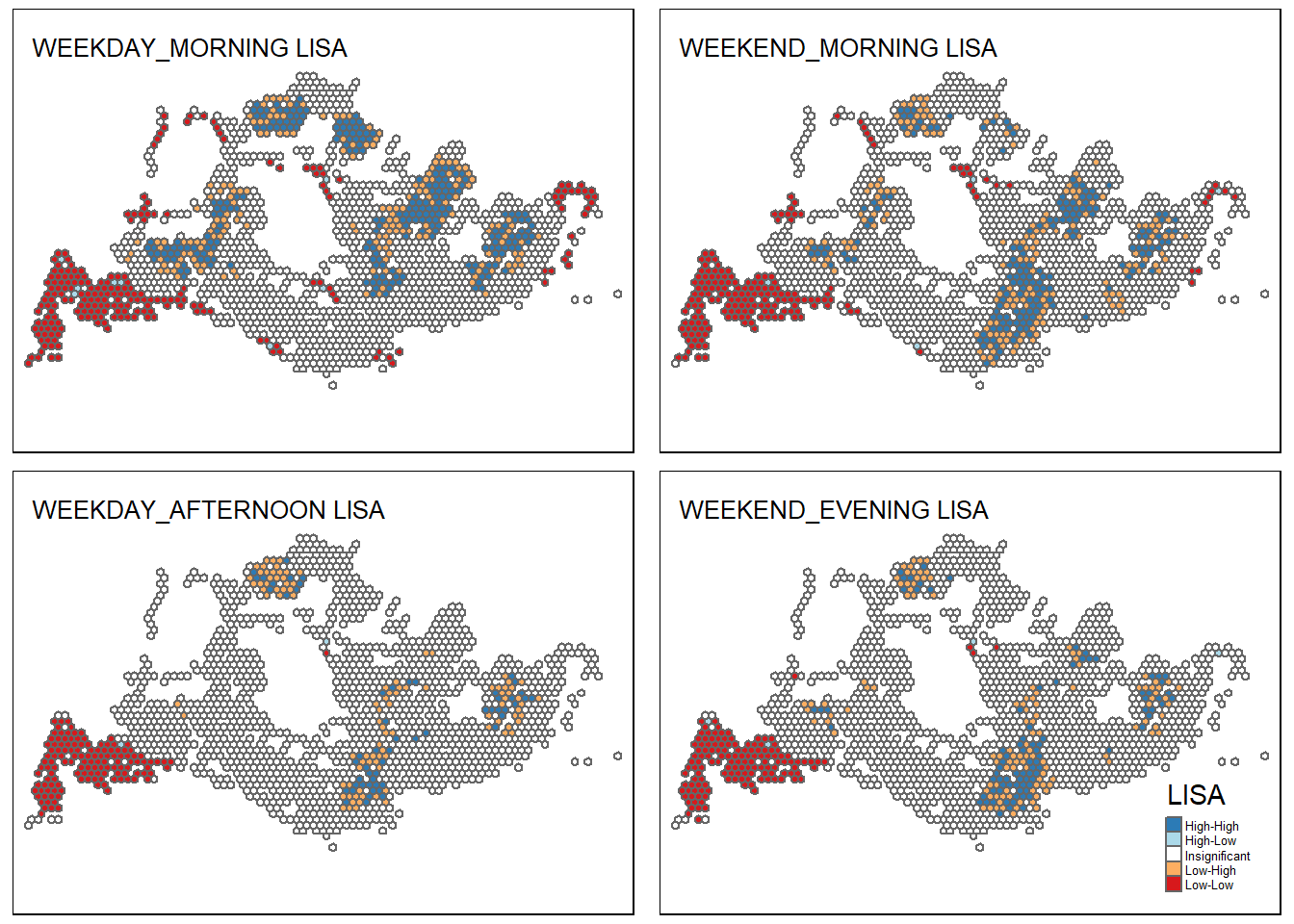
3.7 Plotting the Local Moran’s I statistics
- For completeness, we have also plotted the map of Local Moran’s I statistic for brief discussion;
- We simply wish to observe that there appear to be persistent hotspot hexagons with outlier values (i.e. very positive or very negative) that persist across all peaks.
show code
tmap_mode("plot")tmap mode set to plottingshow code
wd_morn_lmi <- tm_shape(df) +
tm_fill("DAY_MORN_LMI",
palette = "RdBu",
midpoint = 0,
title="Local Moran's I") +
tm_borders() +
tm_layout(title = "WEEKDAY_MORNING", title.size = 0.8,
legend.text.size = 0.4, legend.position = c("left", "top"),
title.position = c("right", "top"))
wd_aft_lmi <- tm_shape(df) +
tm_fill("DAY_AFT_LMI",
palette = "RdBu",
midpoint = 0) +
tm_borders() +
tm_layout(title = "WEEKDAY_AFTERNOON", title.size = 0.8, legend.show = FALSE,
title.position = c("right", "top"))
we_morn_lmi <- tm_shape(df) +
tm_fill("END_MORN_LMI",
palette = "RdBu",
midpoint = 0) +
tm_borders() +
tm_layout(title = "WEEKEND_MORNING", title.size = 0.8, legend.show = FALSE,
title.position = c("right", "top"))
we_eve_lmi <- tm_shape(df) +
tm_fill("END_EVE_LMI",
palette = "RdBu",
midpoint = 0) +
tm_borders() +
tm_layout(title = "WEEKEND_EVENING", title.size = 0.8, legend.show = FALSE,
title.position = c("right", "top"))
tmap_arrange(wd_morn_lmi, we_morn_lmi, wd_aft_lmi, we_eve_lmi)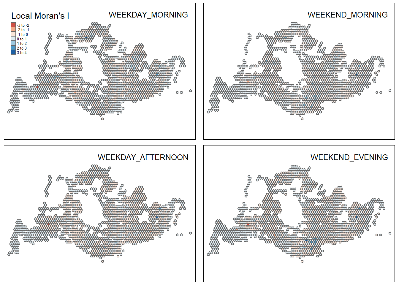
4 Summary Of Observations & Future Work
- From the geospatial visualisations, we have identified regions of high traffic based on bus stop origin trip data.
- Considering only passenger trips (Section 2), there are certain regions where many trips originate. These are likely areas of transit from other transporation types, e.g. MRT Stations or taxi stands.
- Considering LISA (Section 3), there appear to be different traffic demands at different peak times. In particular, we saw a difference in traffic demand regions during Weekday Morning and Weekday Afternoon peaks.
- For further work, we can consider the following:
- Integrating data from other sources of public transport including MRT data. This will provide a more holistic picture.
- Incorporate Emerging Hotspot Analysis across the months and across the hours of the day, in order to get a clearer picture of travel patterns
- Mapping regions of residence/commerce/study in order to provide context for major areas of high traffic.
