In-class Exercise 2: Spatial

GLSA

Getting Started - Import packages

This function calls pacman to load sf, tidyverse, tmap, knitr packages;

• tmap : For thematic mapping; powerful mapping package
• sf : for geospatial data handling, but also geoprocessing: buffer, point-in-polygon count, etc
  • batch processing over GIS packages; can handle tibble format
• sfdep : creates space-time cube, EHSA; replaces spdep
• tidyverse : for non-spatial data handling; commonly used R package
• knitr : generates html table

pacman::p_load(tmap, sf, sfdep, tidyverse, knitr)

Loading the data

• Hunan: geospatial dataset in ESRI shapefile format
  • use of st_read() to import assf data.frame
    • $geometry column is actually a list inside the df cell; that’s the power of the tibble dataframe
    • “features” of simple features refers to geometric features eg point line curve etc
  • note projection is WGS84; see `88
• hunan2012: attribute format in csv format
  • use of read_csv() astbl_df data.frame
• !IMPORTANT! to retain geometry, you must left join to the sf dataframe (eg you can also hunan2012 right join hunan)
  • without sf dataframe, normal tibble dataframe will drop the geometry column

show code

hunan <- st_read(dsn = "data/geospatial", 
                 layer = "Hunan")

Reading layer `Hunan' from data source 
  `C:\1darren\ISSS624\In-class_Ex\In-class_Ex2\data\geospatial' 
  using driver `ESRI Shapefile'
Simple feature collection with 88 features and 7 fields
Geometry type: POLYGON
Dimension:     XY
Bounding box:  xmin: 108.7831 ymin: 24.6342 xmax: 114.2544 ymax: 30.12812
Geodetic CRS:  WGS 84

show code

hunan2012 <- read_csv("data/aspatial/Hunan_2012.csv")
hunan_GDPPC <- left_join(hunan,hunan2012)%>%
  select(1:4, 7, 15)

Plot a chloropleth of GDPPC

show code

#qtm(hunan, "GDPPC") +
#  tm_layout(main.title = "GDPPC", main.title.position = "right")


tm_shape(hunan_GDPPC) +
  tm_fill(col = "GDPPC", 
          style = "pretty",
          palette = "Blues",
          title = "GDPPC") +
  tm_borders(alpha = 0.5) +
  tm_layout(main.title = "GDPPC",
            inner.margins = c(0.1, 0.1, 0.1, 0.1),
            outer.margins = c(0.1, 0.1, 0.1, 0.1)
            ) + 
  tm_grid(alpha = )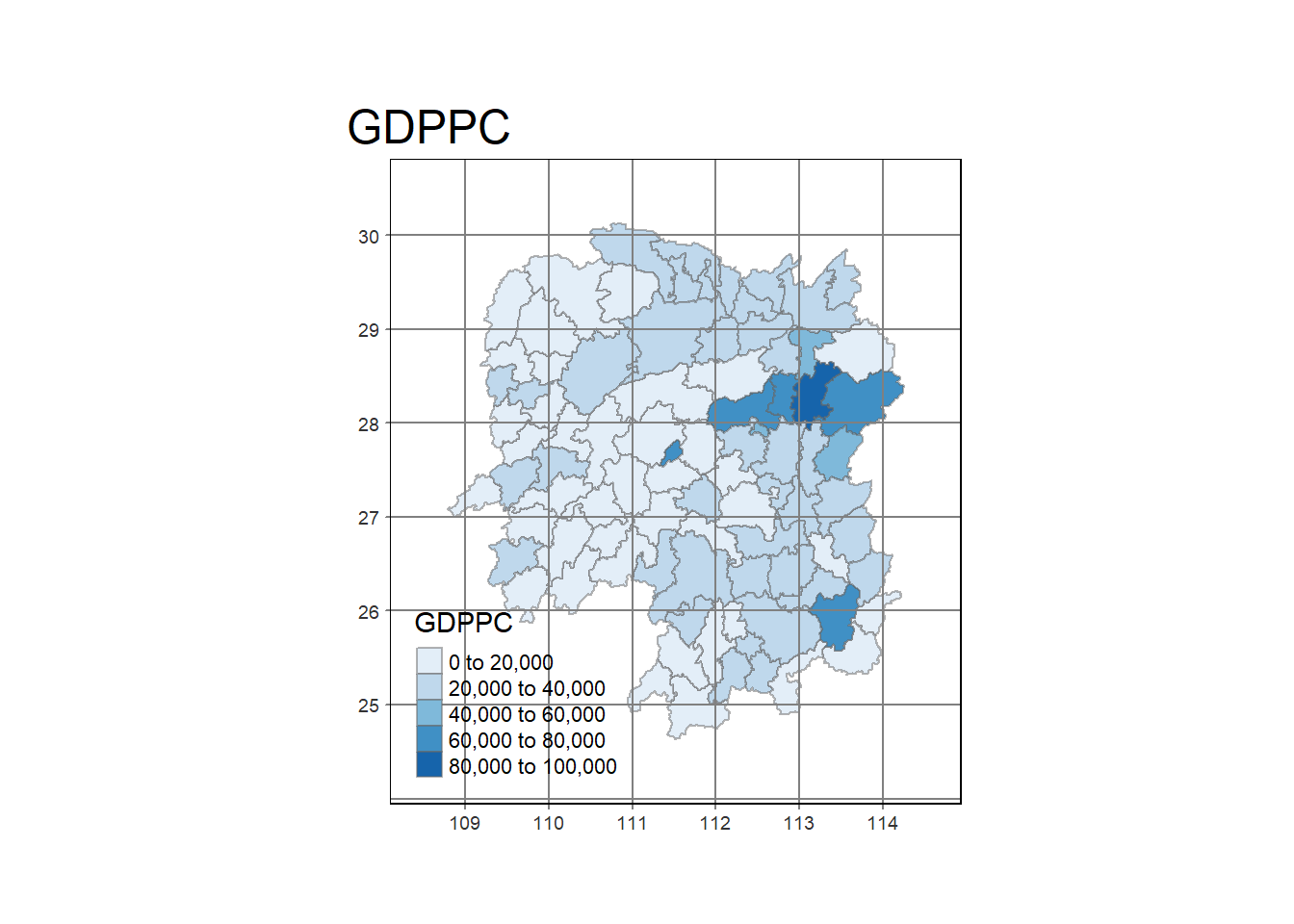 

Deriving QUEEN contiguity weights

• mutate is function that creates new column from previous column datas
  • st_contiguity creates nb neighbour matrix (QUEEN contiguity, by default)
  • st_weights creates row-standardised weights (style="W") from nb object
  • One-step function using sfdep; a wrapper for spdep but writes output into sf dataframe

show code

wm_q <- hunan_GDPPC %>%
  mutate(nb = st_contiguity(geometry), 
         wt = st_weights(nb, style = "W"),
         .before = 1)

Computing Global Moran’s I

• below is “old_style”

show code

# moran_i = global_moran(
#   hunan_GDPPC$GDPPC,
#   hunan_GDPPC$nb,
#   hunan_GDPPC$wt
# )
# glimpse(moran_i)

Computing Local Moran’s I

• Monte Carlo: simulation more accurate, calculate Local Moran’s I using
• unnest is needed to turn the output of local_moran into individual columns in lisa
  • local_moran will create a group table; a separate list of columns that’s hard to read
• several high/low options for Moran’s I
  • $mean is default;
  • $median can be used if distribution is highly skewed (eg skew high == biased to right)

show code

# 
# lisa <- wm_q %>%
#   mutate(localmoran = local_moran(GDPPC, nb, wt, nsim=99), 
#          .before = 1) %>%
#   unnest(localmoran)
# glimpse(lisa)